More GPU adventures with lightGBM

In the meantime the new desktop system has arrived and I installed Tensorflow and Keras for its 1080 Ti. It took me almost a day, because of the slightly different authorization settings it sometimes refused to do things or lost the PATH settings… Actually the biggest problem was that the CUDA tool set version 8 had vanished from the NVIDIA site and that the Tensforflow version does not yet work with version 9. Forunately I kept a copy of the installation files on the laptop…

Finally I had to install Keras from the githug version, the CRAN version did not work for me.

Although it looks even more formidable, setting up lightGBM with GPU support is actually easier.  Okay, this is for the R package and windows 10.  I assume you have already installed the support for the graphical processor,.

I followed the instructions here: http://lightgbm.readthedocs.io/en/latest/Installation-Guide.html but some things need clarification.

Download Visual Studio 2017. Select the free community edition and the first 3 options. Install. Well, thta,s not enough, you need more. Go to the control panel for apps, and change the visual studio installer. On the right hand site it gives you a new list of options. Do download them all – I do not know which ones are essential but this worked for me.

Next download the appropraite boost libabry and install it. Find CMake and install it. If you do not have GIT install that too. Nowyou are ready to go.  Select a directory in which you want to install the lightGBM github sources and run in that directory the commands that are mentioned in step 4 of the above link.

Then start-up Rstudio (or R), set as working directory the R-package directory of the above lightgbm directory and run devtools::install().

This will install lightGBM as a standard R package but without GPU support.  For the GPU support just replavce the lightgbm dll in the R package libs directory with the (larger) version in the lightgbm/release directory.

Now to use it within R you have to add device = “gpu” to the parameters.

 

 

Tensorflow on the GTX 1050

I have a Windows 10 laptop with a GEFORCE GTX 1050. On the NVIDIA developers site it is NOT listed as being supported by the CUDA tools, and therefore, I first assumed, I would not be ble to run GPU supported tensorflow on this machine. However that was a mistake: it is possible and the speed improvement is impressive.

1. Download the CUDA 8.0 toolkit from https://developer.nvidia.com/cuda-downloads
2. Install it, without the drivers, ignore the error message that says it does not see a supported GPU
3. Also download and install the patch from the above website.
4. Create a (free) developers account on the developers site.
5. Download cudNN 6.0 after logging in. Also download the installtion guide.
6. Copy the cudNN files to the location C:\Program Files\NVIDIA GPU
   Computing Toolkit\CUDA\v8.0
7. Check whether the Path for CUDA has been set (see the installation guide if you do not know how to do that).

That’s it. Very simple but it took me hours to figure out.

In R, now you can download the keras package and issues the commands:

libabry(keras)
install_keras(tensorflow="gpu")

and you are ready to rock.

In the first test I ran it was 213 second without gpu and 18 sec with GPU sopprt.

What is a Grnn? Not a neural net!

In a recent article ([1] , [2]) a type of neural net called a Generalized Regression Nueral Net was used. What is it? It turned out to be no more than a simple smoothing algoritm. In the following code my variables that start with a Caapital letter are vectors or matrices. I can write the whole “GRNN” in three lines of R- code :

My_grnn <-
  function(Y, Xtrain, Xtest, sigma, m=nrow(Xtrain)){
    D<- as.matrix(dist(rbind(Xtrain, Xtest)))[1:m, -(1:m)]
    W<- exp(- D^2/((2*sigma^2)))
    return( Y %*% W / colSums(W))
}

Here Xtrain are observation with known results Y, and Xtest are observation for wchich we want to return the predicted values. In this simple algoritm D are the Euclidian distances between Xtrain and Xtest, W is the weight attached to those distances and then we can return the weighted average of Y as predicions.

As an algorithm this does not deserve the name neural network. It is also doing very badly as a machine learning algorithm compared to other generalized regressions. Compare it to the workhorse xgboost on the Boston Housing data.

# ------------- real example
require(MASS)
data(Boston)
B <- scale(Boston, center=TRUE, scale = TRUE)
B[,14]<- Boston[,14]
# the medv column has median value of owner-occupied homes in $1000
# 506 rows,lets take 80 to predict
set.seed(17*41)
h<- sample(nrow(Boston), 80)

Xtrain<- as.matrix(B[-h, -14])
Ytrain<- B[-h, 14]
Xtest<- as.matrix(B[h, -14])
Y_test<- B[h, 14]

# determine best sigma for grnn
range <- seq(0.1, 3, by=0.01)
result <- sapply(range, function(s){
  Y_hat<- My_grnn(Ytrain, Xtrain, Xtest, sigma=s)
  return(Metrics::rmse(Y_hat, Y_test))
})
best<- range[which(result==min(result))]
pred_grnn <- My_grnn(Ytrain, Xtrain, Xtest, sigma=best)

require(xgboost)
param <- list(
  eta = 0.005,
  subsample = 0.95,
  max_depth = 6,
  min_child_weight = 1,
  colsample_bytree = 0.7,
  nthreads = 3
)

dmodel <- xgb.DMatrix(as.matrix(Xtrain), label = Ytrain, missing=NA)
dvalid <- xgb.DMatrix(as.matrix(Xtest), label = Y_test, missing=NA)

model <- xgb.train(
  data = dmodel,
  nrounds = 10000, 
  params = param,  
  watchlist = list(val = dvalid),
  early_stopping_rounds = 1
)
pred_xgb <- predict(model, dvalid, ntree_limit = model$best_iteration)
## compare predictions with root mean squared error
Metrics::rmse(pred_grnn, Y_test)
Metrics::rmse(pred_xgb, Y_test)
## [1] 6.086455
## [1] 2.993994
## yes -- grnn is very bad, a factor 2 worse than xgboost

Notes

[1] J. Abbot & J. Marohasy,  “The application of machine learning for evaluating anthropogenic versus natural climate change”, GeoResJ, dec. 2017,  https://doi.org/10.1016/j.grj.2017.08.001

[2] For fundamental criticism see f.i.  https://andthentheresphysics.wordpress.com/2017/08/22/machine-unlearning/

Why validation in Principle Components Analysis?

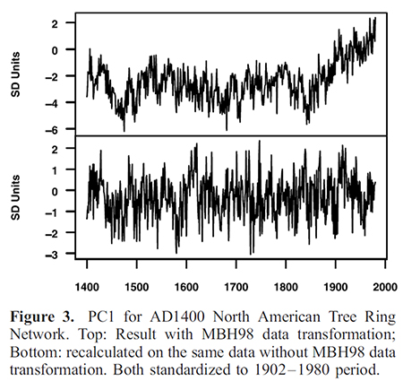
I have written an analysis and replication of the following figure in M&M05:

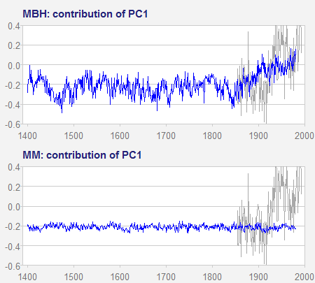
It is known – in some circles- that this figure is misleading. What I have not seen yet is that the figure should have looked like this:

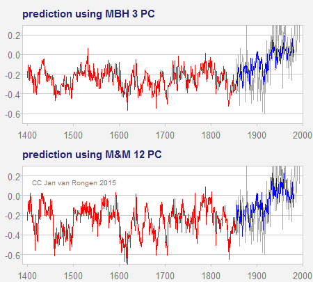
and also not have seen is that – had M&M done a proper validation of the choice of Principle Components, they would also have found a hockestick in their version of the scaling of the data:

The full report is here (warning, PDF):

Draft: Why validation in Principle Components Analysis?

Reactions that are directly related to the statistics and R code in this draft are welcome.  If you have someting else to say wait until after the first revision.

[M&M05a]: McIntyre, S. and McKitrick, R.: 2005, ‘Hockey sticks, principal components, and spurious significance’, Geophys. Res. Lett. 32, L03710

Where was that “hiatus”?

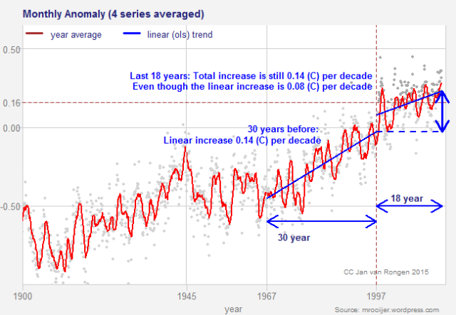
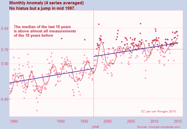
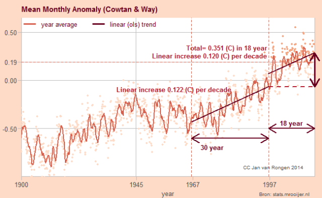
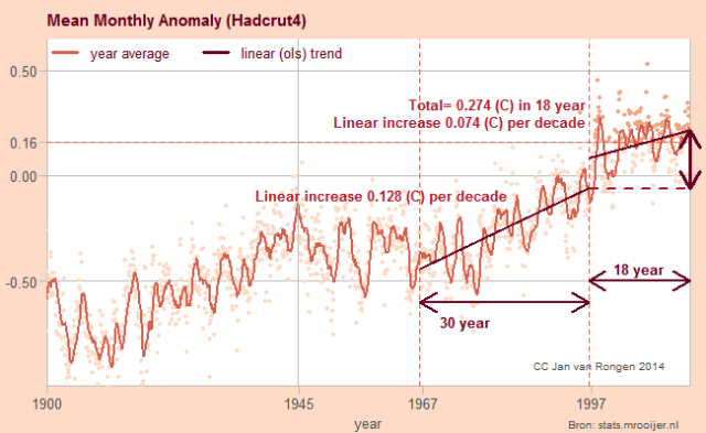
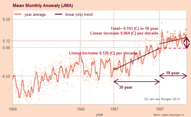
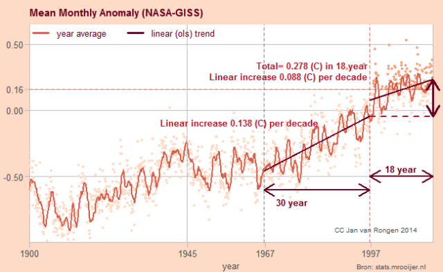
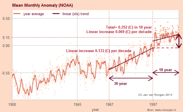
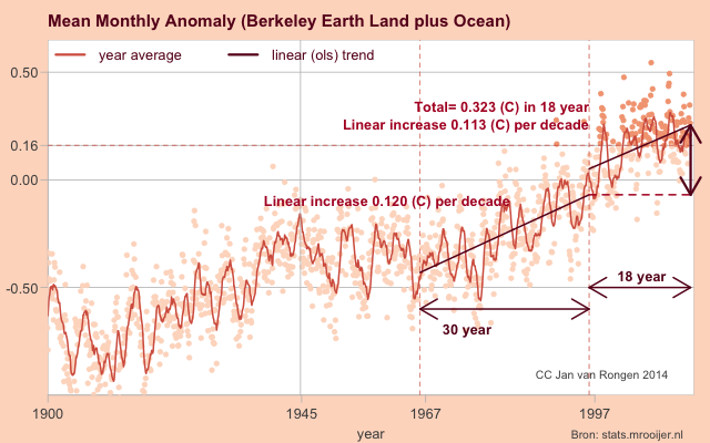
Some people are still believing that the global temperature somehow has not increased, or increased less than expected in the last 18 years. Nothing is further from the truth: taking the average of the four most commonly used surface temperature series (GISS, NCEI, Hadcrut, JMA) until mid 2015 we get the following picture:

Yes, the last 18 years the linear increase was less than the increase in the 30 years before, but that does not mean the overall rise in global temperature anomaly was smaller: there is also this jump that needs to be taken into account. If we do that, the total increase is very consistently 0.14 degrees per decade since 1967.

Let’s zoom in on the upper right corner, it contains an extra message:

 The median of all anomalies since mid 1997 lays .16 above the chosen reference temperature (the average of 1986 – 2006),  but what is astonishing is thathalf of the months in the last 18 years have been warmer than any month before (with two exeptions). .

Takens Theorem

A famous dynamical system is the Lorenz butterfly. It is a curve that moves in time through the (X,Y,Z)-space and that is attracted by a strange attractor.

# discrete simulation of the Lorenz system
# N is some large number

s = 10; r = 28; b = 8/3
x = 1; y=-1; z = 10

dt=0.0075
X=rep(x,N); Y=rep(y, N); Z=rep(z, N)
for (t in 2:N) {
  x=X[t-1];y=Y[t-1]; z=Z[t-1]
  dx= - s*x + s*y
  dy= r*x - y - x*z
  dz= - b*z + x*y
  X[t]=x+dx*dt; Y[t]=y+dy*dt; Z[t]=z+dz*dt  
}

This can be visualized quite easily:

lorenz002 from MrOoijer on Vimeo.

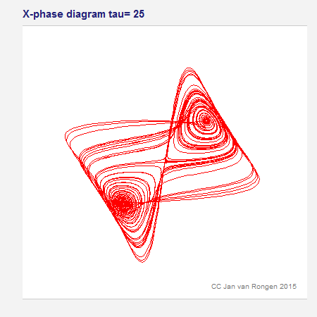
This seems rather chaotic, but there is order in the chaos. There is a theorem by Floris Takens from 1981 that says we can reconstruct the dynamical system from the X-values alone. Choose a parameter tau, and the system (X(t), X(t-tau), X(t-2*tau)) is some kind of projection of the original system. For instance for tau=25 it looks like this:

So let’s assume we have a time series with observations from a system that might be approximated by some dynamical system. Using Takens theorem we can try to understand some of the characteristics of the underlying dynamical system. Or, if we have observed more than one variable, this analysis might help us understand the relationship bewteen the variables.

There are technical difficulties. Takens theorem is about smooth differential equations, whereas in the real world we will observe discrete points in time, i.e. we have difference equations. Secondly, we have a lot of noise in the observations, so we need some sort of stochastic version of the theorem.

Fortunately most of these points have been addressed in the mathematical literature since 1981. See part II.

18 years hiatus?

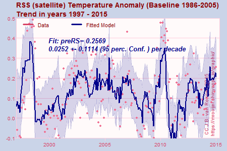
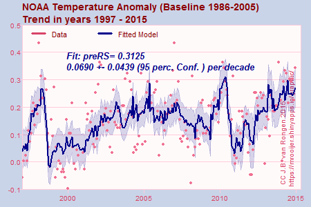
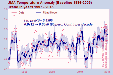
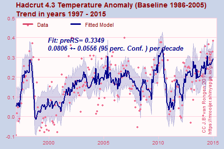
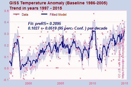
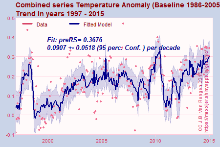
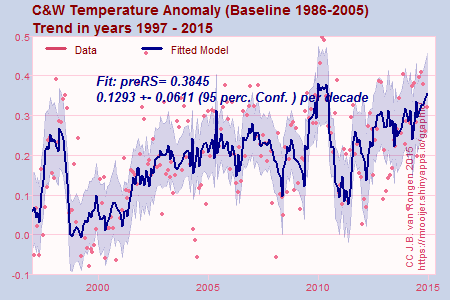
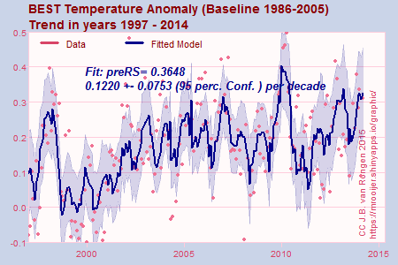
Regression is:

Anomaly= a+ b*(months since 1-1-1997)/120 + 
         c*ENSO(lag=3) + d*TSI(ssp-proxy with lag=3) 
         + e*volcanic_areasols(lag=6)

The confidence intervals are the standard CI’s  corrected for auto-correlation. Notice the larger uncertainty in the coefficients for the satellite-data,  caused by higher auto-correlation and bigger swings in the data.

The preRS is similar to the normal RS but penalizes for variates that do not contribute to the regression enough.

Pictures and processing from https://mrooijer.shinyapps.io/graphic/

Global Temperature Applet

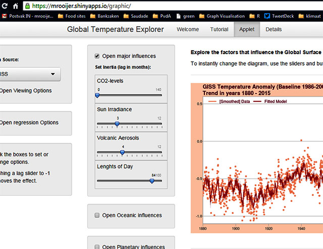
I made an applet in R with Shiny: explore the global temperature trends and the various factors that influence the variations.  Click the picture below to go to the applet.

This is a work in progress. Comments, questions, etc. can be given in the reply area for this blog item.

It has not stopped

And finally the series until end 2013 from Berkeley:

 

GISS Global temperatures: reporting history

GISS Global Sea and Land Surface Temperatures as they were reported in 1981, 1995, 2003 and today. The line are 5 years averages, or, more accurate, 60 months averages.

Sources:

• 1981: Hansen e.a (image copy)
• 1995: Steve Mcintyre (monthly anomaly)
• 2003: Internet Archive (monthly anomaly)
• 2014: current GISS site (monthly anomaly)

Baselines: for 1981 the baseline is the period of 1880-1980. For others it is 1951-1980. Can be found in the documents.

Conclusion: this diagram shows that Steven Goddard erred here.

The “hiatus”

In this picture we have plotted the 60-months moving average against a background of the monthly averages.

If we want to view this moving average as an indication of the current anomaly, then we have to move it to the right, otherwise the moving averages of the “current anomaly” would contain future values.

Normally the hiatus is illustrated by drawing a straight line from around 1997, and – as this line is almost horizontal -it is used as proof that the warming has stalled. However, it is not so simple. In 1997-1998 the global temperatures suddenly rose to new levels, and from that new level indeed the temperatures stayed more or less the same(*).

Look at the dots in the upper right corner. These higher values are all in a sudden  common after 1998, whereas before 1997 there are none of them except for a couple of outliers. After 1998 more than 50% of all months were warmer than any month before (except those 2 outliers).

What we witness is a steep increase of 0.18 degree C in 5 years time followed by a stationary period. You cannot call that a stagnation IMHO. The next blog item gives a more detailed analysis.

(*) Using only values after 1997 in an autocorrelated series is a statistical blunder.